BCI Classification Performance Calculator
Confusion Matrix
Evaluation of Classification Performance
In BCI applications, as in other applications of classifiers, it is important to evaluate the accuracy and the generalization performance of a chosen classifier. Here, we will have a look at some of the major evaluation techniques.Confusion matrix
When evaluating performance, it is useful to find out members of the confusion matrix. For binary (true or false) problems this matrix is of size 2 x 2. Four entries in the matrix correspond to:- TP (true positives) - the number of correct positive classifications
- FN (false negatives) - the number of missed positive classifications
- FP (false positives) - the number of incorrect positive classifications
- TN (true negatives) - the number of correct rejections
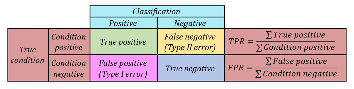
Figure 1: Confusion matrix components. There are four possible outcomes from a binary classifier.
If the outcome from a prediction is p and the actual value is also p, then it is called a true positive (TP); however, if the actual value is n then it is said to be a
false positive (FP). Conversely, a true negative (TN) has occurred when both the prediction outcome and the actual value are n, and false negative (FN) is when the prediction
outcome is n while the actual value is p.
ROC space
When we vary some characteristic of the classifier, for example, threshold, we obtain different numbers of true positives and true negatives. A plot of the proportion of true positives(TPR, true positive rate) versus the proportion of false positives(FPR, false positive rate), when some parameter of the classifier (for example threshold) is varied, is known as a ROC curve ("receiver operating characteristic curve, a term with origins in signal-detection theory). Figure 2 illustrates where different types of classifiers fall in the ROC space. Confusion matrices for this data points with calculated TPR and FPR can be found in figure 3.
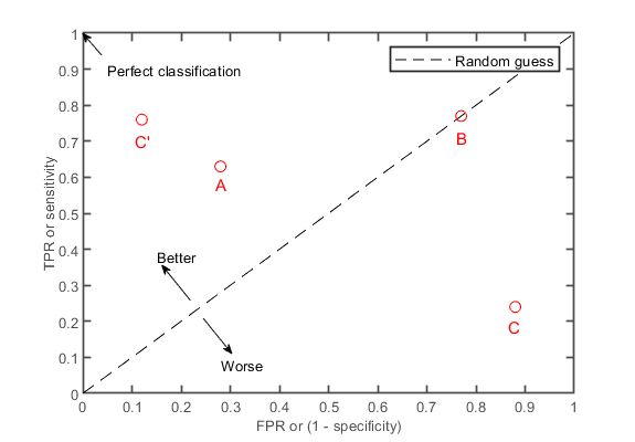
Figure 2: The ROC space. The TPR defines how many correct positive results occur among all positive
samples available during the test. FPR, on the other hand, defines how many incorrect positive results occur among all negative samples available during the test. A and C'
are classifiers that perform that chance (random guessing) whereas B performs at chance levels. C performs significantly worse than chance. The perfect classifier occupies
the top left corner and has TPR of 1 and FPR of 0. Ideally, we would like our classifier to be as close to the top left corner as possible.
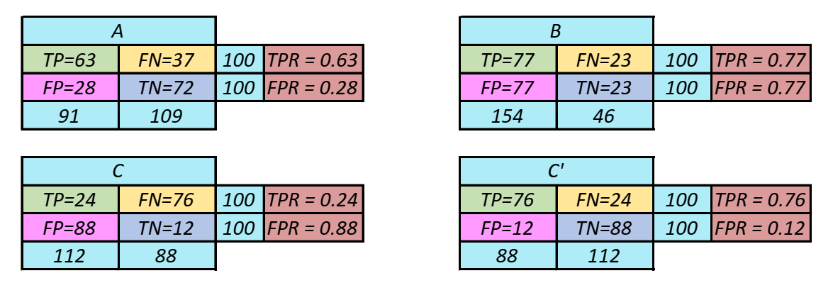
Figure 3: Results of classifiers. These results are plotted on the ROC space above.
Classification Accuracy
The classification accuracy \(ACC\) is defined as a ratio between correctly classified samples and the total number of samples. It can be derived from the confusion matrix M as follows: $$ACC = {TP+TN \over TP+FN+FP+TN}$$ When the number of examples for each class is the same, the chance level is \(ACC_0 = {1 \over N_Y}\), where \(N_Y\) denotes the number of classes (2 for binary classifier).Kappa Coefficient
Kappa coefficient is another useful performance measure. $$k = {ACC-ACC_0 \over 1-ACC_0}$$ The kappa coefficient is independent of the samples per class and the number of classes. \(k = 0\) means chance level performance and \(k = 1\) means perfect classification. \(k < 0\) means that classifier perform at worse than chance level.Logo - Design - Scripts by Margret Stilke-Volosyak.
1 Wolpaw, Jonathan, and Elizabeth Winter Wolpaw, eds. Brain-computer interfaces: principles and practice. OUP USA, 2012.
2 Rao, Rajesh PN. Brain-computer interfacing: an introduction. Cambridge University Press, 2013.